Computational Fluid Dynamics (CFD)

Computational Fluid Dynamics

   Introduction

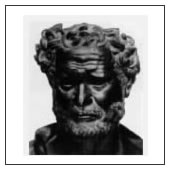
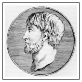
A Brief History of CFD Since the dawn of civilization, mankind has always had a fascination with fluids; whether it is the flow of water in rivers, the wind and weather in our atmosphere, the smelting of metals, powerful ocean currents, or the flow of blood around our bodies. Heraclitus 536 - 470BC Archimedes 287 - 212BC In antiquity, great Greek thinkers like Heraclitus postulated that "Everything flows" but he was thinking of this in a philosophical sense rather than in a recognizably scientific way. However, Archimedes initiated the fields of static mechanics, hydrostatics, and determined how to measure densities and volumes of objects. The focus at the time was on waterworks: aqueducts, canals, harbors, and bathhouses, which the ancient Romans perfected to a science. 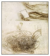It was not until the Renaissance that these ideas resurfaced again in Southern Europe when we find great artists cum engineers like Leonardo Da Vinci starting to examine the natural world of fluids and flow in detail again. He observed natural phenomena in the visible world, recognizing their form and structure, and describing them pictorially exactly as they were. He planned and supervised canal and harbor works over a large part of middle Italy. 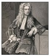His contributions to fluid mechanics are presented in a nine part treatise (Del moto e misura dell'acqua) that covers water surfaces, movement of water, water waves, eddies, falling water, free jets, interference of waves, and many other newly observed phenomena Leonardo Da Vinci's sketches of objects and free surface effects in water Sir Isaac Newton 1643 - 1727 Leonardo was followed in the late 17th Century by Isaac Newton in England. Newton tried to quantify and predict fluid flow phenomena through his elementary Newtonian physical equations. His contributions to fluid mechanics included his second law: F=m.a, the concept of Newtonian viscosity in which stress and the rate of strain vary linearly, the reciprocity principle: the force applied upon a stationary object by a moving fluid is equal to the change in momentum of the fluid as it deflects around the front of the object, and the relationship between the speed of waves at a liquid surface and their wavelength. 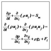In the 18th and 19th centuries, significant work was done trying to mathematically describe the motion of fluids. Daniel Bernoulli (1700-1782) derived Bernoulli's famous equation, and Leonhard Euler (1707-1783) proposed the Euler equations, which describe the conservation of momentum for an inviscid fluid, and conservation of mass. He also proposed the velocity of potential theory. Two other very important contributors to the field of fluid flow emerged at this time; the Frenchman, Claude Louis Marie Henry Navier (1785-1836), and the Irishman, George Gabriel Stokes (1819-1903) introduced viscous transport into the Euler equations, which resulted in the now-famous Navier-Stokes equation. These forms of the differential mathematical equations that they proposed nearly 200 years ago are the basis of the modern-day computational fluid dynamics (CFD) industry, and they include expressions for the conservation of mass, momentum, pressure, species, and turbulence. Indeed, the equations are so closely coupled and difficult to solve that it was not until the advent of modern digital computers in the 1960s and 1970s that they could be resolved for real flow problems within reasonable timescales. Other key figures who developed theories related to fluid flow in the 19th century were Jean Le Rond d'Alembert, Siméon-Denis Poisson, Joseph Louis Lagrange, Jean Louis Marie Poiseuille, John William Rayleigh, M. Maurice Couette, Osborne Reynolds, and Pierre Simon de Laplace. Claude Navier A simplified form of the Navier-Stokes equations George Stokes In the early 20th Century, much work was done on refining theories of boundary layers and turbulence in fluid flow. Ludwig Prandtl (1875-1953) proposed a boundary layer theory, the mixing length concept, compressible flows, the Prandtl number, and much more that we take for granted today. Theodore von Karman (1881-1963) analyzed what is now known as the von Karman vortex street. Geoffrey Ingram Taylor (1886-1975) proposed a statistical theory of turbulence and the Taylor microscale. Andrey Nikolaevich Kolmogorov (1903-1987) introduced the concept of Kolmogorov scales and the universal energy spectrum for turbulence, and George Keith Batchelor (1920-2000) made contributions to the theory of homogeneous turbulence.         It is debatable as to who did the earliest CFD calculations (in a modern sense) although Lewis Fry Richardson in England (1881-1953) developed the first numerical weather prediction system when he divided physical space into grid cells and used the finite difference approximations of Bjerknes's "primitive differential equations". His own attempt to calculate whether for a single eight-hour period took six weeks of real-time and ended in failure! His model's enormous calculation requirements led Richardson to propose a solution he called the "forecast-factory". The "factory" would have involved filling a vast stadium with 64,000 people. Each one, armed with a mechanical calculator, would perform part of the flow calculation. A leader in the centre, using coloured signal lights and telegraph communication, would coordinate the forecast. What he was proposing would have been a very rudimentary CFD calculation. The earliest numerical solution for flow past a cylinder was carried out in 1933 by Thom and reported in England A.Thom, ‘The Flow Past Circular Cylinders at Low Speeds', Proc. Royal Society, A141, pp. 651-666, London, 1933 Kawaguti in Japan obtained a similar solution for flow around a cylinder in 1953 by using a mechanical desk calculator, working 20 hours per week for 18 months! M. Kawaguti, ‘Numerical Solution of the NS Equations for the Flow Around a Circular Cylinder at Reynolds Number 40', Journal of Phy. Soc. Japan, vol. 8, pp. 747-757, 1953. During the 1960s, the theoretical division of NASA at Los Alamos in the U.S. contributed many numerical methods that are still in use in CFD today, such as the following methods: Particle-In-Cell (PIC), Marker-and-Cell (MAC), Vorticity-Stream function methods, Arbitrary Lagrangian-Eulerian (ALE) methods, and the ubiquitous k - e turbulence model. In the 1970s, a group working under D. Brian Spalding, at Imperial College, London, developed Parabolic flow codes (GENMIX), Vorticity-Stream function based codes, the SIMPLE algorithm, and the TEACH code, as well as the form of the k - e equations that are used today (Spalding & Launder, 1972). They went on to develop Upwind differencing, 'Eddy break-up', and 'presumed pdf' combustion models. Another key event in the CFD industry was in 1980 when Suhas V. Patankar published " Numerical Heat Transfer and Fluid Flow", probably the most influential book on CFD to date, and the one that spawned a thousand CFD codes. It was in the early 1980s that commercial CFD codes came into the open market place in a big way. The use of commercial CFD software started to become accepted by major companies around the world rather than their continuing to develop in-house CFD codes. Commercial CFD software is therefore based on sets of very complex non-linear mathematical expressions that define the fundamental equations of fluid flow, heat and materials transport. These equations are solved iteratively using complex computer algorithms embedded within CFD software. The net effect of such software is to allow the user to computationally model any flow field provided the geometry of the object being modelled is known, the physics and chemistry are identified, and some initial flow conditions are prescribed. Outputs from CFD software can be viewed graphically in colour plots of velocity vectors, contours of pressure, lines of constant flow field properties, or as "hard" numerical data and X-Y plots. CFD is now recognized to be a part of the computer-aided engineering (CAE) spectrum of tools used extensively today in all industries, and its approach to modelling fluid flow phenomena allows equipment designers and technical analysts to have the power of a virtual wind tunnel on their desktop computer. CFD software has evolved far beyond what Navier, Stokes or Da Vinci could ever have imagined. CFD has become an indispensable part of the aerodynamic and hydrodynamic design process for planes, trains, automobiles, rockets, ships, submarines; and indeed any moving craft or manufacturing process that mankind has devised.

Computational fluid dynamics or CFD analysis is one of the key analysis methods used in engineering applications. The origins of CFD lies in mankind’s efforts to better understand the power of natural elements like wind, storms, floods, or sea waves.

Mesh Generation:

Mesh or grid is defined as a discrete cell or elements into which the domain/ model is divided. All the flow variables & any other variables are solved at centers of these discrete cells. This entire process of breaking up a physical domain into smaller sub-domains (elements/ cells) is called as mesh generation.

Why we need a Mesh?

Basically, a mesh is required because by physics or mathematical theory we are solving the variables like flow and heat transfer and any other variable at these cell centers or nodes.  Also, the theoretical methods that are used for any CFD study like the fine difference method (FDM), finite element method (FEM) and the finite volume method (FVM) actually solve the variable at these discrete cells/ nodes.

There are different types of grid/ cell shapes e.g. triangles, quadrilateral, tetrahedral, hexahedra, etc, that will we see in detail. for e.g. the image below shows a glimpse of a CFD random mesh between two circles, the domain of analysis. We have filled the space (torus) by many small triangles called cells or elements. A grid or mesh is a collection of all these triangles.

Here the point that needs to be noted is that the mesh composed of many triangles are always connected with each other, however, they never intersect with each other.

The domain inputs that would be needed for solving the equation are:

1. Appropriate shape & size of the domain in which the equation will be solved.
2. The domain needs to be discretized as it will be given to the solver for solving the equation is discretized form.
3. Domain & boundary tags (boundary conditions); making sense of physics.
4. Write output file needed for the solver.

Meshing Terminologies:

1. Cells & element types: The cells & elements shapes should be supported by the used solver. Typical cell shapes supported by commercial solvers (ANSYS Fluent, ANSYS CFX) are of following types:

• For 2-D elements: 
  

• For 3-D elements:

Types of Grid / Mesh:

The typical types of grid/ mesh used for commercial software for academic or industrial applications are:

1. Cartesian 
2. Structured
3. Unstructured
4. Hybrid

The mesh generally may not always consist of a single type of elements viz., triangles or rectangular blocks, etc. Sometimes we need to use different meshing techniques to shape the model in order to capture the shape of a particular CAD model. The mesh elements therefore at the same time may consist of cartesian, structured, unstructured & hybrid mesh. Within the structured grid, we have mono-block & multi-block type of mesh. Mono-block & multi-block meshing are the processes we follow to get a structured type of mesh. Within the unstructured grid, we have triangular tetrahedron & with Hybrid grid, we have a mix of above-discussed elements.

1. Cartesian Grid:

Cartesian grid means that the entire set of discrete cells that we will be using in order to fill the CFD space are aligned along the orthogonal axis, i.e. alignment along the x, y & z-axis. eg. as below:

This facilitates the use of square or rectangles/ cubes, the most simple form of the mesh but it does not capture the shape exactly & hence used rarely. Also, the result obtained with this will not be that accurate & typically used for a very simple type of geometries.

2. Structured Grid:

Here a single block is used to cover the entire geometry. Also used for simple shapes, where a single block is sufficient for covering the CAD model.

e.g. a cylinder

In a Structured Mesh, elements are aligned in a specific manner or they follow a structured pattern & hence the name structured mesh. Conversely, if the elements are arranged in a random fashion or haphazardly they are called un-structured mesh.

2.1. Structured Mono-Block Grid: 

For preparing a structured mesh a single bounding block is used to cover the entire geometry. Also used for simple shapes where a single block is sufficient for actually covering the entire CAD model.

In order to generate mesh for the cylinder (example below), we can cover the cylinder with a bounding box that can be a single bounding box & then generate the mesh for entire cylinder, called a mono-block since a single bounding block is used for generating the mesh.

Within structured mesh, the other method we use to mesh a complex geometry is called a multi-block. Let us say, if suppose in the core of cylinder we want to generate a finer mesh or a different pattern compared to the outer region, thus to separate this we at times use more than one bounding box (figure below). Similarly, for a complex geometry like the catalytic converter, we cannot cover the shape by a single bounding box so we generate different bounding box for different shapes within the same CFD space & then combining these blocks we make a single structured mesh. Since there are multiple blocks involved in the mesh generation process this is called multi-block structured mesh.

3. Unstructured Grid: 

It is the entire discrete cells we generate within the CFD space are randomly spaced & do not follow any single pattern & hence the name un-structured mesh. The types of unstructured mesh are shown in figure below:

Triangular/ Tetrahedron

Quadrilateral/ Hexahedron:

4. Hybrid Grid:

Most of the complex meshing process used to study complex geometries as shown in the figure below. The top part of the image has squares and triangles i.e. tetrahedrons & hexahedrons in volume. Since the shape/ geometry is complex we cannot capture the shape profile by using a single element type, hence we use multiple types so we use triangles, prisms, wedges as well as a hexahedron. Similarly, for volume mesh of a sphere along the sphere surface, we use tetrahedron and inside we use hexahedron. Thus a combination of different shapes gives us a hybrid mesh.

Coming up next, Grid Generation for CFD Simulations:

Reference: